SYSTEM DESIGN:Lesson 3: Do the Math on a Napkin

The question that separates "I read a blog" from "I have shipped"

"How many servers do you need for 10 million daily active users?" The interviewer is not looking for a precise answer. They want to see you reason with numbers instead of hand-waving.

Back-of-envelope estimation is the skill of getting within an order of magnitude of the right answer in five minutes, using a pen, a whiteboard, and round numbers. No calculator app. No Google.

Every system design interview at Flipkart, Google, or a Series B startup will ask you to estimate QPS, storage, or bandwidth. We start with a URL shortener — the same problem you will design in Lessons 7–8 — then give you reference tables and a second worked example you can adapt to any product.

Back-of-envelope math on a coffee-stained napkin

The napkin is optional. The panic is not.

Start here: URL shortener napkin math in 5 minutes

If you are prepping the URL shortener design, do this section first. Say these numbers out loud in the interview before you draw boxes. Round aggressively — within 2× is fine.

Assumptions (negotiate with the interviewer)

New short links per day:     100 million
Read:write ratio (redirects): 100:1
Bytes per row (code + URL):  ~600 bytes
Retention horizon:           10 years (optional but impressive)
Peak multiplier:             3× average (lunch + evening)

Writes — creating short links

100M / day ÷ 100K sec/day ≈ 1,000 writes/sec average
Peak (3×):                  ~3,000 writes/sec

One Postgres primary handles that. Writes are not the scary part for a URL shortener.

Reads — redirects

1,000 writes/sec × 100 = 100,000 reads/sec average
Peak (3×):               ~300,000 reads/sec
One viral IPL link (10× on one code): CDN + Redis absorb most of this

This is why URL shorteners are read-heavy. Cache and CDN are not optional at scale — they are the design.

Storage — how much disk in 10 years

100M/day × 365 days × 10 years ≈ 365 billion rows
365B rows × 600 bytes ≈ 220 TB raw (before replicas)
With 3× replication:        ~660 TB

You do not need a calculator in the room. You need the shape: modest writes, huge reads, linear disk growth.

Bandwidth — redirects are tiny

Peak read QPS: 300,000
301 redirect response: ~500 bytes (headers + Location)
Outbound ≈ 300K × 500 B = 150 MB/sec ≈ 1.2 Gbps
CDN (95% hit): origin sees ~75 MB/sec — manageable

Sanity check — does this pass the smell test?

Memorize this one example. When the interviewer says "design a URL shortener," you already have four numbers on the board before minute five. Full design walkthrough: Lesson 4 and Lessons 7–8.

The sections below are reference material — powers of 2, latency, formulas, and a second worked example (social feed). Come back when you need them for other problems.

Powers of 2: the cheat code for storage math

Storage and memory are measured in powers of 2. You do not need to calculate them — you need to recognize them instantly.

The shortcut: add 3 zeros for every 10 in the exponent.

2^20 ≈ 10^6  (million)
2^30 ≈ 10^9  (billion)
2^40 ≈ 10^12 (trillion)

When someone says "we store 500 GB of user photos," you should instantly think: that is roughly 500 × 2^30 bytes, or about 5 × 10^11 bytes. If each photo averages 2 MB, that is about 250,000 photos. The math takes 15 seconds once you know the table.

Time conversions to memorize:

Round aggressively. "About 100K seconds in a day" is close enough for any interview. Precision to the third decimal place impresses nobody.

Latency numbers every engineer should know

Estimation is not just about storage and QPS. You need to know how long things take — because a design that requires 50 sequential network calls will never feel fast, no matter how many servers you add.

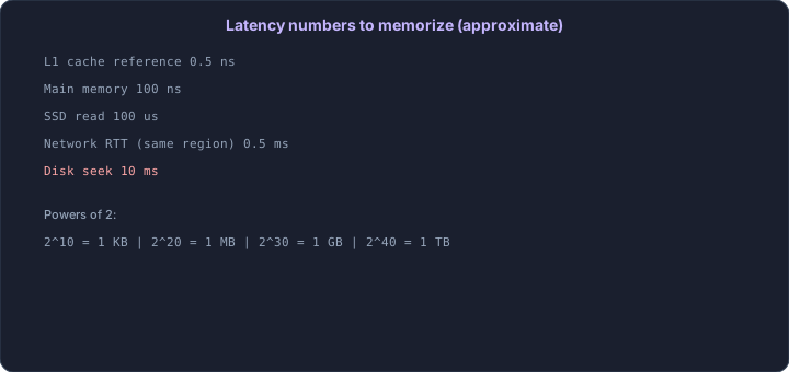
Latency cheat sheet from L1 cache to cross-continent RPC

The insight that changes how you design:

Memory is 100,000x faster than disk. Redis is 10x faster than Postgres. A same-datacenter call is 100x faster than a cross-country one. Every time you add a network hop, you add milliseconds. Design accordingly.

Budget for a 200ms API response:
  Load balancer:        1 ms
  App server logic:     5 ms
  Redis cache lookup:   1 ms
  Postgres query:       10 ms
  Serialization:        2 ms
  Network to client:    50 ms (India mobile)
  ─────────────────────────
  Total:               ~70 ms  ✓ well within budget

Same request with 5 sequential Postgres queries:
  5 × 10 ms = 50 ms just in DB → 110 ms total → getting tight

This is why caching matters. This is why you batch database queries. This is why putting your servers in Mumbai for an Indian user base is not optional.

QPS: the number that drives everything

Queries Per Second (QPS) — or Requests Per Second (RPS) — is the heartbeat of system design. Almost every capacity decision flows from this number.

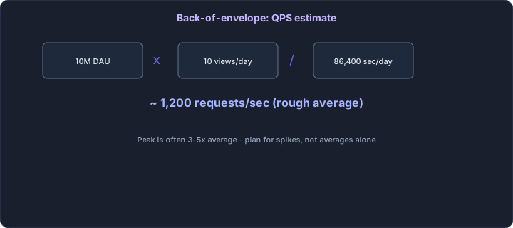
QPS estimation flow from DAU to peak requests

The formula:

Daily requests = DAU × requests per user per day
Average QPS  = daily requests / 100,000  (seconds in a day, rounded)
Peak QPS     = average QPS × peak multiplier

Peak multiplier rule of thumb:

Quick example:

Product: Twitter-like app in India
DAU: 10 million
Requests per user per day: 100 (scroll feed, post, like, refresh)

Daily requests = 10M × 100 = 1 billion
Average QPS    = 1B / 100K = 10,000
Peak QPS (3x)  = 30,000

30,000 QPS is a serious number. You need load-balanced app servers, read replicas, caching, and probably a CDN. A single server handles maybe 1,000–5,000 QPS depending on request complexity. You need at least 6–30 app servers at peak.

Read vs write QPS:

If read:write ratio is 100:1 and total QPS is 30,000:
  Read QPS  = 29,700
  Write QPS = 300

This split tells you where to invest: 29,700 reads/sec screams for caching and read replicas. 300 writes/sec is manageable on a single well-tuned primary database.

Storage estimation: how much disk do you need?

The formula:

Total storage = number of records × size per record × replication factor
Annual growth = daily new records × size per record × 365

Example — photo-sharing app:

Users: 50 million
Photos per user per year: 200
Average photo size: 2 MB
Replication factor: 3 (primary + 2 replicas)

Annual photos = 50M × 200 = 10 billion
Raw storage     = 10B × 2 MB = 20 PB
With replication = 20 PB × 3 = 60 PB per year

60 PB per year is Instagram-scale. For a startup, you would estimate 1% of that in year one and plan S3 with lifecycle policies to move old photos to cheaper storage tiers.

Text data is cheap. Media is expensive.

Always ask: is this text or media? A billion text records is a database problem. A billion photos is a storage architecture problem.

Bandwidth estimation: the number everyone forgets

The formula:

Bandwidth = QPS × average response size

Example:

Peak QPS: 30,000
Average API response: 10 KB

Outbound bandwidth = 30,000 × 10 KB = 300 MB/sec = 2.4 Gbps

2.4 Gbps outbound is significant. A single 1 Gbps network interface saturates at ~100 MB/sec. You need multiple NICs or a CDN to absorb image and video traffic.

CDN impact on bandwidth:

Without CDN: 2.4 Gbps hits your origin servers
With CDN (90% cache hit): 0.24 Gbps hits origin → 10x reduction

This is why every Indian consumer app uses CloudFront or Cloudflare. The bandwidth math alone justifies the CDN cost.

Worked example: design a social feed for 50M DAU

Let us estimate everything for a Twitter/X-like social feed targeting the Indian market. This is the kind of problem you get in a 45-minute system design interview.

Step 1 — Clarify assumptions

DAU:                    50 million
Posts per user per day:   2
Feed refreshes per day:   50
Followers per user (avg): 200
Post size:                500 bytes (text + metadata)
Feed page size:           20 posts × 500 bytes = 10 KB
Read:write ratio:         25:1
Peak multiplier:          3x

Step 2 — Calculate QPS

Writes per day  = 50M users × 2 posts   = 100M
Reads per day   = 50M users × 50 refreshes = 2.5B
Total per day   = 2.6B requests

Average QPS = 2.6B / 100K = 26,000
Peak QPS    = 26,000 × 3 = 78,000

Write QPS (peak) = 78,000 / 26 = 3,000
Read QPS (peak)  = 75,000

Step 3 — Calculate storage

Posts per day:     100 million
Storage per day:   100M × 500 bytes = 50 GB/day
Storage per year:  50 GB × 365 = ~18 TB/year
5-year retention:  ~90 TB
With 3x replication: ~270 TB

Step 4 — Calculate bandwidth

Read bandwidth (peak) = 75,000 QPS × 10 KB = 750 MB/sec = 6 Gbps
Write bandwidth (peak) = 3,000 QPS × 500 bytes = 1.5 MB/sec

Step 5 — Capacity plan

App servers:    75,000 read QPS / 2,000 per server = ~40 servers (with headroom: 60)
Redis cache:    Hot feed for active users, ~20 GB memory
Read replicas:  3 replicas handling 25,000 QPS each
Primary DB:     3,000 write QPS — needs careful indexing, possibly sharding
CDN:            Offload media, reduce origin bandwidth by 90%

Step 6 — Sanity check

The write QPS of 3,000 is the number to flag in an interview. It is fine today with a well-tuned primary, but you should mention sharding as a future consideration when writes exceed 5,000/sec.

Estimation shortcuts for interviews

Memorize these. They save you three minutes every time.

1 million users × 10 requests/day = 10M requests/day ≈ 100 QPS average
10 million users × 100 requests/day = 1B requests/day ≈ 10,000 QPS average
100 million users × 10 requests/day = 1B requests/day ≈ 10,000 QPS average

1 server ≈ 1,000–5,000 QPS (depends on request complexity)
1 Postgres primary ≈ 1,000–10,000 write QPS (depends on query complexity)
1 Redis instance ≈ 100,000 ops/sec
1 GB RAM ≈ 1 million small cached objects

The 80/20 rule for estimation:

Spend 80% of your time on the biggest number. For a photo app, that is storage. For a payment app, that is write QPS and consistency. For a feed app, that is read QPS and bandwidth. Identify the elephant first.

Common estimation mistakes

Mistake 1 — using monthly active users instead of daily.

MAU is typically 3–5x DAU. Estimating QPS with MAU overcounts by 3–5x. Always clarify: "I will assume DAU unless you say otherwise."

Mistake 2 — forgetting the peak multiplier.

Average QPS of 10,000 sounds manageable. Peak QPS of 50,000 during an IPL match is not. Always calculate peak.

Mistake 3 — ignoring response size in bandwidth.

A JSON API returning 1 KB vs a feed returning 50 KB changes your bandwidth estimate by 50x. Ask about payload size.

Mistake 4 — precise numbers when rounding is fine.

Saying "86,400 seconds per day" instead of "about 100K" wastes time and adds no credibility. Round aggressively, state your assumptions, move on.

Mistake 5 — estimating servers without accounting for headroom.

If you need 40 servers at peak, plan for 60. Servers fail, deployments roll, traffic grows. 50% headroom is standard.

What comes next: the interview framework

You now have the numbers. The next chapter gives you the process — a 4-step framework and a 45-minute timeline for system design interviews.

Continue here: System Design Interview Framework.